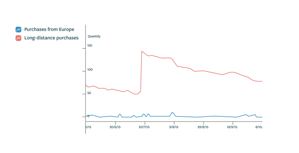
Product manufacturing has rarely been as inexpensive as it is today. At the same time, transportation costs for those products are at record highs. The main reason for this shift is the growth of mass importation from low-cost countries, especially East Asia.
There has long been a trade-off between distance and cost. When goods are purchased from halfway around the world, the factory gate prices may be lower, but long and unreliable delivery times increase costs and supply chain risks. At worst, delayed deliveries or inaccurate demand forecasting may lead to product shortages and stock-outs. Safety buffers are required when delivery schedules are extended and unreliable, which increases the need for storage space.
There are debates in supply chain management circles, sometimes quite heated, about the costs of long-distance procurement for many trading businesses. But there’s no need to get hot under the collar. Instead, I’d encourage companies to reap benefits from both short- and long-distance procurement by using them in combination. Manufacturing businesses already know how to identify and manage supply chain risks related to sourcing. It is time for companies that can handle long-distance, long-lead buying to level up their supply chain management game, improve their sales forecasting, and buy better!
In this article, I will:
- Compare the procurement costs for long and short delivery times and give guidelines for making comparisons.
- Present the best aspects of both procurement models to drive simultaneous benefits.
- Discuss the requirements for utilizing a combined operations model.
Costs associated with long delivery times
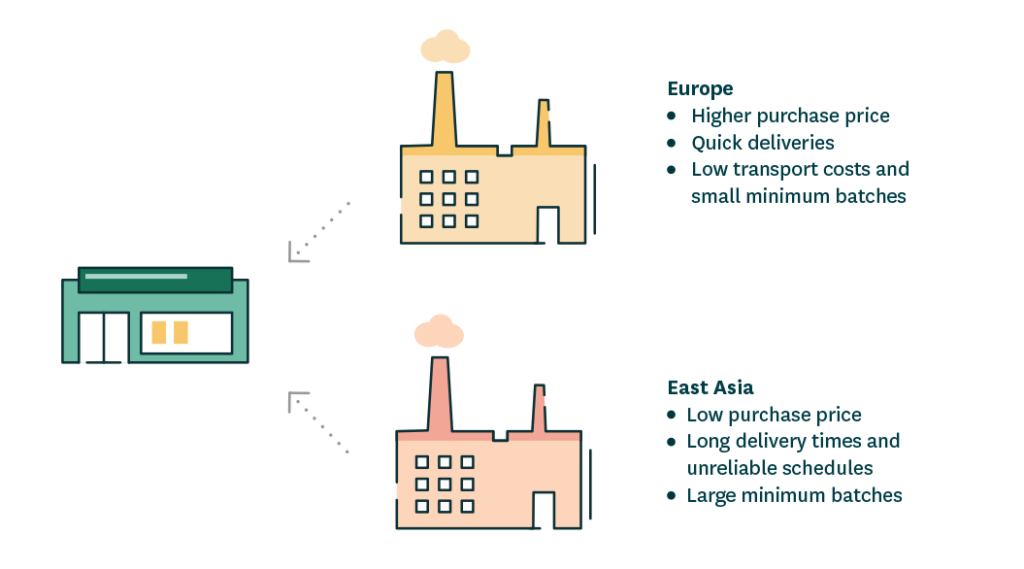
The main driver for using a remote supplier rather than a local one is the lower purchase price. When East Asian manufacturers or wholesalers sell goods for considerably lower prices than their European or American counterparts, the difference can be enormous, even considering the higher transportation costs. That price difference could have a crucial impact on a retailer’s profitability.
However, prolonged and unreliable delivery schedules significantly increase inventory management costs, as more storage space and capital are required. Further, demand forecasting becomes harder the shorter the product’s life cycle, and the risk of receiving unsalable products rises as delivery times get longer. Retailers rarely consider a product’s total procurement cost when selecting a source and seldom consider it when assessing its ultimate profitability. However, they can calculate an indicative cost in advance.
Example 1: Long-distance vs short-distance procurement
Let’s compare a product costing €100 from Europe, with delivery paid for by the supplier, and one costing €60 from East Asia, with the delivery charges covered by the buyer. The product is not particularly large or heavy.
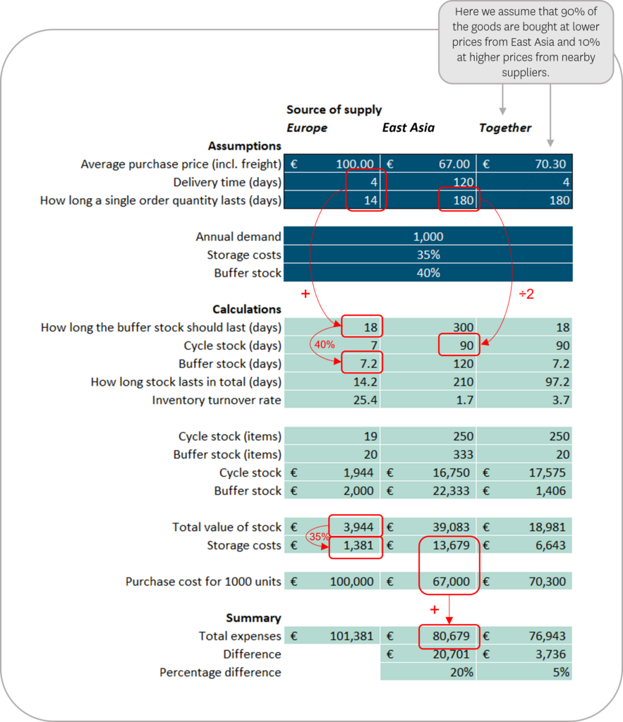
When the product is transported in full units, the comparable purchase price from East Asia is €67, translating into a difference of €33 in the procurement price alone. However, the minimum purchase batch sourced from East Asia covers six months of demand, while it’s feasible to buy just two weeks’ supply from the European source.
For our example product, assume that a buffer stock of approximately 40% of the average sales per purchase cycle is needed (and maintained) to ensure availability. Factoring storage space expenses, interest on capital, and the risk of being left with excess stock, the total costs for storage come to 35% of the purchase price.
In our example, the storage costs for the product from East Asia are ten times those of buying from Europe. When goods are purchased from Europe, the inventory turnover rate is slightly over 25, while the equivalent figure for procurement from Asia is only 1.7. Nonetheless, the total costs for procurement from East Asia are still 20% lower.
Based on cost alone, buying a product from East Asia is more profitable if the purchase price is at least 17% lower than the price offered by a European supplier. If the price difference is less, using the European supplier will eventually be cheaper.
The above calculations are explained in Appendix 1: Explanation of the calculation examples and can be used to create a cost comparison spreadsheet for any business.
Long-distance purchases have increased risks, especially when sales forecasting cannot accurately predict demand. If demand is higher than expected or delivery schedules slide, products may sell out before the next delivery arrives, resulting in unhappy customers and lost sales. Moreover, suppose sales are lower than expected. In that case, products – especially items with a short life cycle – may have to be discounted or destroyed, increasing costs and decreasing the product margin.
In a fluctuating market, the risks of long-distance sourcing are higher than usual. When a company buys enough products to cover six months’ sales and keeps a regular buffer stock, it’s within the realm of possibility that it could find itself with enough stock for 300 days. If sales drop radically, that inventory could hang around for years.
Because of the uncertainties inherent in long-distance procurement, I suggest companies take advantage of the best aspects of long-distance and short-distance procurement.
The best of both worlds: Using long- and short-distance suppliers
Utilizing long-distance and short-distance procurement in parallel improves delivery reliability, increases supply chain management flexibility, and lowers overall costs.
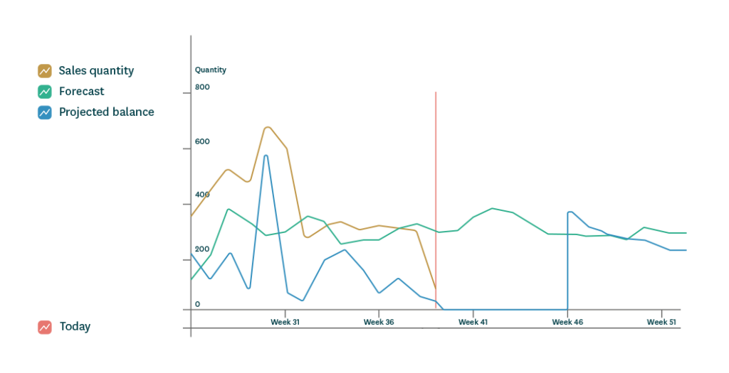
Let’s assume East Asia will remain our product’s primary supply channel. However, finding an alternative supplier that is more local increases flexibility. To reap the benefits of this approach, you need to start with projected sales. Those projections will drive the proportion of the estimated stock requirement you should purchase from the cheaper but more distant supplier. You also need to consider minimum order quantities, shipping consolidation, door-to-door delivery times, etc. The local supplier then acts as a buffer against unexpected demand surges when the trade-off between a higher price but quicker delivery and smaller order quantities shifts in its favor.
However, to make this system work, there needs to be continuous monitoring of actual sales against forecasts, availability, stock levels, and incoming and outgoing deliveries. Monitoring is the easiest if your procurement planning system can give you advanced warning of possible availability problems. If sales are higher than predicted or deliveries are delayed, you can purchase enough goods from the local supplier to mitigate the risk of shortages.
Sea freighting items from China to Europe typically takes 30 to 50 days. If you have only two weeks’ stock in hand and your order from China only left Shanghai one day previously, you will likely need the product to cover a minimum two-week gap. Because you can solve such availability problems utilizing a nearby supplier, you can optimize the buffer stock based on delivery times.
Example 2: Combined operations model
We’ve established that the product in the previous example is purchased primarily from Asia, but unexpected circumstances necessitate backup orders for about 10% of the annual volume.
In this case, the combined operations model would ensure better availability levels while keeping total costs 5% lower than long-distance procurement alone. The inventory turnover rate also rises from 1.7 to 3.7. These benefits will soon appear in improved key logistics figures and decreased stock pressure which increases the resiliency of the supply chain – at a lower cost. Also, reducing the need for high buffer stock levels will decrease dead stock over time. The economic benefits will be highest for products where sales are the hardest to predict.
Assuming procurement and logistics expenses account for 65% of our example company’s turnover and 50% of the goods are purchased from long-distance suppliers, 5% cost savings for these products will translate into savings of 1.5% of the turnover, and thus a 1.5% increase in business profits.
The same model can be used dynamically during the product life cycle or for a particular sales period. Fashion giant Zara does precisely that. For new lines, Zara generally turns to nearby sources because, in the more fashion-driven end of the apparel industry, sales forecasting has historically struggled to predict demand. Should a product begin to sell well, purchasing will shift to larger quantities from lower-cost sources.
Supply channels with shorter delivery times are used again at the end of the product life cycle to avoid surplus stock. However, it may be challenging for companies not working on Zara’s scale to create such a model, depending on their sector.
Simple in theory
Unfortunately, as with many other inventory management ideas, while the principle behind using both long- and short-distance procurement is clear and even relatively simple, making the supply chain operations model work on a large scale is considerably more challenging. However, if you tackle the challenge systematically and purposefully, it is entirely feasible.
The most fundamental practical issue is the increased inventory management workload resulting from the necessity of finding alternate suppliers. An additional challenge arises because purchase volumes will still be uncertain during negotiations. In addition to realized sales, the volumes depend on the reliability of the primary supply source. Therefore, various wholesale companies are generally a natural choice as secondary suppliers.
When product volumes are large, it is also essential that data systems can support the chosen operations model. Of course, every trading company looks for alternative product suppliers and makes backup purchases. However, in the target operations model, potential shortages are identified in advance, triggering a pre-determined sequence of events. If the process can be implemented directly in the system, the only thing remaining is the selection of alternative suppliers and the maintenance of the supplier information. Additionally, the system must be able to integrate forecasting and manage the varied suppliers’ requirements, such as order quotas.
Getting started: Take sure steps at a suitable speed
The process of implementing a model with two sources of supply should be a gradual one. I recommend identifying and prioritizing essential products – those at the core of the selection with large sales quantities. These are the products for which an existing backup supplier is most critical to manage risks and ensure customer satisfaction.
Nearly all industrial companies try to guarantee the availability of their crucial components by using several suppliers. In this respect, wholesale and retail companies have fallen behind. Only when the availability of key products has been ensured is it time to start simply optimizing costs. Cost cutting should begin with products whose sales volumes cannot be easily predicted and have a short life cycle. The new model should be implemented first for the products with the most significant sales volumes—the greater the unpredictability and the larger the sales volumes, the greater the benefits.
Appendix 1: Explanation of the calculation examples
- All figures are for illustrative purposes and do not represent an actual retailer.
- The annual demand has been stated at 1,000 items, but the relative difference between various sources of supply remains the same, even if demand is higher or lower.
- The buffer stock is a way of preparing for fluctuations in demand – predictions rarely match reality exactly. The buffer stock makes up for fluctuation in demand during the delivery period and order interval.
- In the combination model, the buffer stock is needed only to cover the short-distance supplier’s delivery time and order interval, even if most goods are purchased from the long-distance supplier.
- Average stock quantities (in items) have been calculated by multiplying the number of days the stock lasts by the estimated daily demand (1,000 ÷ 360).
- The figures have been calculated based on average purchase prices.
- Here, the long-distance procurement expenses have been compared to the costs for short-distance procurement (–20%) and expenses under the combination model with those of long-distance procurement alone (–5%).
- Usable stock is the portion of the stock that is needed to cover the predicted sales quantities. The stock quantity depends on the order quantity – the average stock level is half that of a single order plus the buffer stock.