Many companies track impressive-looking metrics yet still face empty shelves, excess inventory, and spoiled produce. It’s not for lack of effort. It’s that traditional accuracy metrics often fail to connect to business outcomes.
In supply chain planning, forecasting is always a means to an end. Effective accuracy measurement reveals where forecast errors actually hurt the business and where they have minimal impact. It identifies which products require improved predictions and which need alternative operational approaches. Most importantly, a good system knows when to stop chasing perfect forecasts and start fixing other parts of the planning process.
Understanding how to measure, interpret, and act on forecast performance separates high-performing retailers and wholesalers from their competitors. The difference lies not in better numbers but in better availability, less waste, optimized inventory, and stronger profits. This guide demonstrates how to use forecast accuracy as a tool for making smarter supply chain decisions.
Key takeaways
- Forecast accuracy alone doesn’t guarantee business success and must connect to actions and KPIs like availability, spoilage, and inventory turnover.
- Different metrics serve different purposes: MAPE for comparisons, bias for systemic errors, and cycle error for replenishment impact.
- Good forecast accuracy varies dramatically by product type, sales volume, and planning horizon.
- It’s best to focus accuracy measurement efforts on areas where they matter most, such as fresh products, high-value items, and volatile demand patterns.
- Modern forecasting methods, such as the RELEX ML-based approach, deliver accuracy improvements over traditional time-series methods.
What is forecast accuracy, and why does it matter?
Forecast accuracy measures how closely demand predictions match actual sales. It informs nearly every store and supply chain decision, from determining how much inventory to hold and when to order to staff scheduling and production capacity.
Poor accuracy creates cascading effects across the business:
- Customer experience suffers when stockouts prevent shoppers from finding what they need.
- Working capital gets tied up in excess inventory, increasing the risk of markdown or spoilage.
- Waste increases for perishables, where over-forecasting leads to unsold goods and under-forecasting causes lost sales.
- Labor efficiency declines when inaccurate forecasts drive overstaffing during slow periods or understaffing during peak demand.
The larger the forecast error, the greater the business impact. For example, even a 10% error for a fresh retailer can mean the difference between profit and loss for entire categories. Over-forecasting by 10% means shelves stocked with fresh salads, berries, and pastries will spoil before they can be sold, generating pure waste. Under-forecasting by the same margin means empty shelves during peak hours and customers choosing alternatives, resulting in lost sales that never return.
Forecast accuracy vs. forecast bias
While often discussed together, forecast accuracy and forecast bias measure fundamentally different things. Both must be tracked to truly understand forecast performance and act accordingly.

Forecast accuracy measures the average size of an error regardless of direction. Whether over-forecasting by ten units or under-forecasting by ten units, the accuracy calculation treats both as the same magnitude of error. This indicates the degree of variability in predictions and shows overall forecasting performance, helping retailers and wholesalers understand the level of uncertainty their planning processes must accommodate.
Forecast bias reveals systematic over- or under-forecasting. If forecasts consistently run 5% high or 5% low, then there’s a bias problem. Bias is expressed as a percentage: results over 100% indicate over-forecasting, while results under 100% indicate under-forecasting. Tracking bias is critical because it detects systemic issues that accumulate over time and across locations.
| Metric | What it measures | How it’s calculated | What it tells us | Common misinterpretation |
| Forecast accuracy | The average size of errors, regardless of whether forecasts over- or under-estimate demand. | Compares absolute error between forecast and actual (direction irrelevant). | Indicates how closely forecasts align overall and how much uncertainty planners must account for. | High accuracy does not mean there is no bias. A forecast can be consistently wrong in the same direction. |
| Forecast bias | Systematic tendency to over- or under-forecast. | Compares forecast to actual as a ratio or percentage (over 100% = over-forecasting; under 100% = under-forecasting). | Highlights structural issues in the forecasting process that compound over time and across locations. | Low bias does not mean a forecast is accurate. It may fluctuate widely around the correct value. |
A small bias at the store or item level can seem insignificant in isolation. But when that same bias is repeated across hundreds of stores or rolled up to a distribution center, it quietly creates major inventory imbalances. Consistently over-forecasting by just 5% means ordering more than needed. Even a 2% bias can tie up capital in excess stock, especially when item-level patterns go unnoticed.
This is where aggregated metrics become misleading. A forecast can appear highly accurate at the total level, even when individual items are consistently over- or under-forecasted.
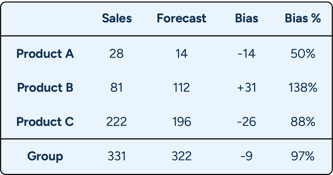
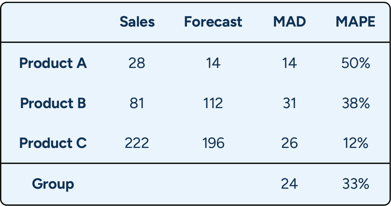
Imagine that three products are forecasted for the same week. At an individual level, each item shows a large forecasting error — some significantly over-forecasted, others under-forecasted. However, when aggregated, these errors largely cancel each other out. The result is a group-level forecast that appears highly accurate, masking substantial item-level bias that would still drive excess stock or missed sales.
What is a “good” level of forecast accuracy?
There’s no universal benchmark for “good” forecast accuracy because no two businesses face the same forecasting conditions. What counts as “good” depends on the uncertainty built into the product mix, demand patterns, and planning horizons —factors that determine what level of accuracy is actually achievable.
Several factors have an outsized impact on realistic accuracy levels:
- Sales volume. High-volume products typically achieve better forecast accuracy because random variation smooths out across larger numbers. Low-volume items are more exposed to day-to-day variability and percentage swings.
- Demand variability. Products with stable, year-round demand are far easier to forecast than those influenced by promotions, seasonality, or irregular spikes.
- Forecast horizon. Short-term forecasts are inherently more reliable, while longer-term forecasts face growing uncertainty.
Typical accuracy ranges vary dramatically by product type:
| Product Type | Typical Range | Why This Range Makes Sense |
| High-volume, stable products | 75–85% | Large volumes smooth out random variation, and demand patterns are predictable. |
| Slow-movers with intermittent demand | 50–70% | Low volume and sporadic demand create large percentage swings, making higher accuracy unrealistic. |
| Fresh products with weather-sensitive demand | 70–80% | External factors introduce inherent volatility, limiting achievable precision even with good models. |
Ultimately, understanding when and why forecast accuracy drops matters more than chasing arbitrary targets.
Key metrics for measuring forecast accuracy
No single metric tells the complete story of forecast performance. The same dataset can yield dramatically different accuracy readings depending on the metric used and the aggregation method employed. A forecast might show 95% accuracy by one measure while simultaneously revealing a 15% error by another, and both could be technically correct.
Each metric addresses a distinct business question, ranging from comparing performance across categories to monitoring how forecast errors impact replenishment decisions. What matters is matching the right metric to the specific planning context and using multiple metrics together to get the full picture.
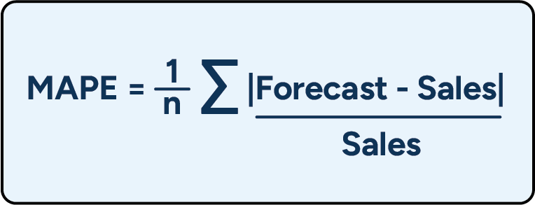
MAPE (Mean Absolute Percentage Error)
Mean Absolute Percentage Error (MAPE) shows, on average, how many percentage points off forecasts are, making it the most widely used metric in demand planning. The calculation compares absolute forecast error to actual sales volume, treating each product or time period equally, regardless of its size.
MAPE works best for comparing forecast performance across different products or categories, as the percentage format is consistent regardless of volume differences.
However, MAPE can produce misleadingly high error percentages for slow-moving products where small absolute errors translate to large percentage swings. It’s also impossible to calculate when actual sales are zero, making it problematic for intermittent demand items at the daily level.
Use MAPE for product mix analysis, category performance reviews, and comparing forecasting performance across different scales.
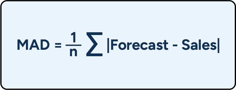
MAD (Mean Absolute Deviation)
Mean Absolute Deviation (MAD) shows the average size of forecast errors in units, making it straightforward to understand but limited in application. While MAPE expresses forecast error as a percentage of sales, MAD calculates the average absolute difference between forecasted and actual sales in the original units.
MAD works best for analyzing single-product forecast performance, particularly when comparing the results of different forecasting models applied to the same SKU. However, because MAD gives the average error in units, it is not particularly useful for comparing across different datasets.
For example, if Model A averages 12 units of error per week for a laundry detergent SKU while Model B averages 8 units, Model B clearly performs better. However, that 8-unit error can’t be meaningfully compared to a different product, such as paper towels, where sales volumes and unit economics are entirely different.
WAPE (Weighted Absolute Percentage Error)
Weighted Absolute Percentage Error (WAPE) compares absolute errors to actual values, assigning more weight to larger values.
The formula for this metric is:
WAPE=t∑wt∣yt∣∣yt−y^t∣
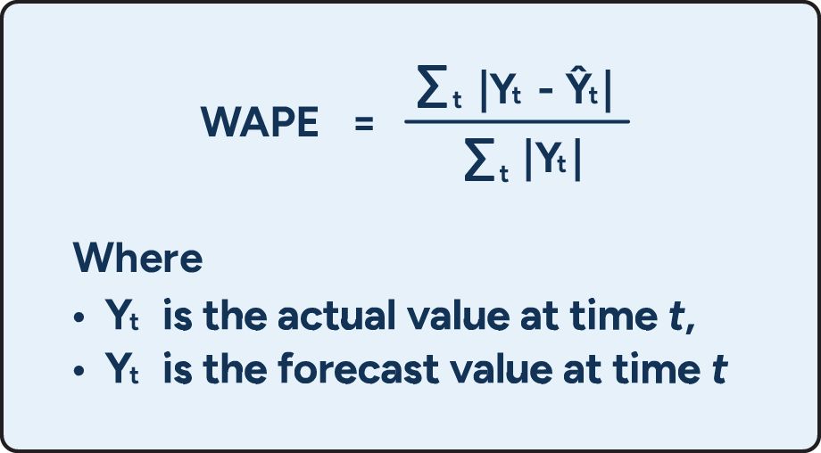
It’s well-suited for measuring overall business performance because it accounts for the relative importance of items by weighting errors based on their sales volume. This prevents distortion caused by slow-moving items, which might otherwise disproportionately impact metrics like MAPE.
WAPE gives more weight to larger sales volumes to provide a realistic view of the overall impact on operations. High-volume products naturally have a greater influence on the metric, reflecting their significance to business outcomes.
While effective at measuring aggregate performance, WAPE can be disconnected from operational impact in specific situations. A product might exhibit poor WAPE accuracy but still perform well operationally if factors such as large batch sizes or infrequent ordering cycles absorb forecast errors.
For example, a product with 15% forecast accuracy (measured as 1-WAPE) might maintain adequate stock levels if replenishment is driven by batch sizes rather than precise daily forecasts. This is why WAPE should be complemented with process-specific metrics that connect accuracy to actual business decisions.
Note: RELEX uses 1-WAPE (expressed as a percentage) as a primary accuracy metric, where a higher percentage indicates better forecast accuracy.
Forecast error and forecast bias in batches
Forecast error and bias in batches are two RELEX-developed metrics that directly connect forecast accuracy to replenishment decisions. These metrics indicate whether forecast errors during order calculation were substantial enough to result in different order quantities than would have been obtained with perfect forecast accuracy. Unlike statistical measures that operate independently of business processes, batch-based metrics show whether forecast inaccuracies actually distort ordering decisions.
The formulas for these metrics are:
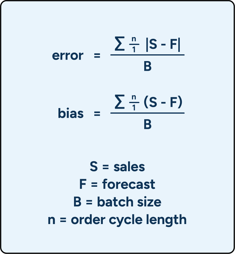
Critically, these metrics are scale-agnostic, meaning the effect on replenishment remains consistent regardless of demand volume. A product selling 0.23 units per day and another selling 230 units can be evaluated using the same thresholds. Percentage-based metrics, such as MAPE, however, require different interpretations depending on product velocity.
Using these metrics provides clear, actionable decision thresholds:
- Cycle error < 0.25: Ordering decisions aren’t affected by forecast inaccuracy—no improvement efforts required
- Cycle error > 1: Forecast inaccuracies are actively distorting optimal order quantities—focus forecasting efforts here, prioritizing products with the highest cycle forecast error
How to measure forecast accuracy
Measuring forecast accuracy effectively requires a systematic approach that aligns measurement methodology with actual business processes. The following five steps establish a robust framework for tracking and interpreting forecast performance.
Step 1: Define measurement scope
Before calculating any metrics, define precisely what’s being measured and why. The scope should reflect how forecasts actually drive operational decisions.
Time horizon
The forecast version used to measure accuracy should match the time lag when important business decisions are made.
For fast-moving consumer goods (FMCGs) and fresh products with short lead times, it is essential to measure forecast accuracy at shorter horizons. This is typically 1-2 weeks in advance for store replenishment or even daily for products with very short shelf lives. Fresh products require particularly tight alignment since forecast errors translate almost immediately into either waste or lost sales.
For long-lead items, such as those sourced from overseas, the relevant measurement horizon extends much further. If a supplier delivers with a 12-week lead time, what matters is the forecast quality when the order was created, not when the products arrived.
These different horizons come with different attainable accuracy levels and planning implications.
- Short-horizon forecasts for FMCG support daily replenishment, where accuracy directly affects availability and waste.
- Long-horizon forecasts for overseas-sourced products guide larger commitment decisions, where factors like flexible sourcing or strategic inventory positioning may matter as much as—if not more than—raw forecast accuracy.
Forecasts naturally become more accurate closer to the sales period, so measuring the wrong version gives a misleading picture of the forecast performance that actually drove decisions.
Aggregation level
The appropriate aggregation level depends entirely on the planning process being supported. Different decisions happen at different levels of granularity, so forecasts should be evaluated at the level where those decisions are made.
The table below illustrates different aggregation level shifts.
| Planning process | Recommended aggregation level | Why this level matters |
| Store replenishment | Store–SKU–day | Ordering decisions occur daily at the store–SKU level. |
| Distribution center inventory planning | DC–SKU–week | Weekly aggregation aligns with how DC inventory is planned and managed. |
| Sales & Operations Planning (S&OP) | Category–month | Strategic decisions require a broader, monthly category view. |
Choosing the wrong aggregation level can distort the interpretation of results, making performance appear better or worse than the accuracy that actually influenced planning decisions. Ensuring alignment between the aggregation level and the planning process is essential for drawing meaningful conclusions about forecast quality.
Product scope
Not all products require the same level of forecast accuracy to drive good business results. Products should be classified based on their importance and predictability. ABC classification reflects economic impact based on sales value, while XYZ classification captures demand variability and forecasting difficulty. Combining them helps determine where accuracy truly matters.
| Segment | Characteristics | Forecast accuracy expectation | Exception thresholds | Why it matters |
| AX (High value, stable demand) | High sales value, high frequency, predictable patterns | High accuracy is realistic and critical | Very low | Drives major revenue and margin outcomes |
| AY / AZ (High value, variable demand) | High value but more volatility | Moderately high expectations | Moderate | Still important financially; volatility requires caution |
| BX / BY / BZ (Medium value) | Moderate contribution and varying predictability | Balanced expectations | Balanced | Important enough to monitor but not worth over-optimizing |
| CX / CY / CZ (Low value) | Low economic impact, often low frequency | Lower expectations | High | Excess scrutiny wastes effort; tolerate more error |
This segmentation ensures that measurement efforts focus on areas where accuracy has the greatest impact on business results.
Step 2: Collect and prepare data
Accurate measurement requires collecting the correct data at the right time and properly cleansing it to reflect actual forecast performance, not supply chain constraints.
Required data
- Historical forecasts at decision time. Collect the forecast version that was active when key business decisions were made. For example, when measuring replenishment performance, the relevant forecast is the one that existed when orders were placed, not the most recent update.
- Actual sales/demand data. Gather actual sales or demand data for the same time periods and aggregation levels as the forecasts.
- Contextual information. Collect data about promotional periods, assortment changes, price modifications, and other planned business decisions that should have been reflected in forecasts. This helps distinguish between forecast model errors and planning process failures.
Data cleansing
Raw sales data requires careful cleansing to ensure it reflects actual demand rather than distortions caused by supply constraints or external factors:
- Remove stockout periods. These artificially depress actual sales figures and make forecasts appear overly optimistic when the real issue was a supply constraint, not a forecast error.
- Adjust for cannibalizations and substitutions. When customers bought alternative items because their first choice wasn’t available, these purchases represent latent demand that should be credited to the original forecast.
- Flag promotional periods. Some metrics behave very differently during promotions versus baseline selling periods.
Step 3: Calculate chosen metrics
After defining the scope and preparing the data, the next step is calculating forecast accuracy metrics. However, the calculation approach itself significantly impacts results, even when using the same underlying data and metric formulas.
Apply formulas at the appropriate aggregation level
Each chosen metric should be calculated at the aggregation level that matches the business process. MAPE, MAD, bias, and cycle forecast error should use the same time buckets and product groupings defined earlier.
It’s also important to stay consistent in how metrics are interpreted. Accuracy metrics target 100%, while error metrics target 0%. Forecast bias, despite its name, is an accuracy metric. MAD and MAPE measure error.
Understand the difference between aggregating data and aggregating metrics
Another important consideration is how aggregation is handled. Metrics can be calculated on aggregated data or calculated at a detailed level and then averaged. Both approaches are valid, but they answer different questions and should never be compared directly.
For example, calculating MAPE on aggregated group-level data may produce a result of 3%. Calculating MAPE at the product level and then averaging those results could yield 33% for the same dataset. Neither is wrong, but each tells a very different story.
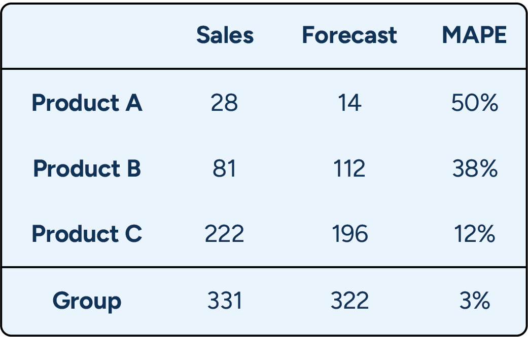
Which number is correct? Both are, but they answer different questions and should never be compared.
From a store replenishment perspective, a 3% error calculated at an aggregated level would be misleading. Replenishment decisions depend on product-level accuracy, where large individual errors are hidden by aggregation.
At a more aggregated decision level, such as planning picking capacity in a distribution center, the same 3% error is far more meaningful. In this case, what matters is total volume accuracy, not how each individual product performs.
Step 4: Interpret results in context
Calculating metrics is only the beginning. Value comes from understanding what those numbers mean for real planning decisions. Accuracy percentages on their own rarely drive action, so results need to be interpreted against the right context to surface meaningful patterns and underlying issues.
Compare to relevant benchmarks
Assess forecast accuracy results against these three reference points:
- Historical performance trends. Monitor results over time to determine whether accuracy is improving, declining, or stable. Early shifts can signal changes in demand patterns.
- Product segment benchmarks. Split results by ABC/XYZ classification or similar segmentation. Attainable accuracy varies widely: high-volume, stable products may reach 85–95%, intermittent items often fall between 50–70%, and fresh, weather-sensitive products typically sit around 70–80%.
- Business impact thresholds. Compare results to thresholds such as cycle forecast error in batches to determine whether inaccuracies actually affect replenishment decisions. This helps separate forecasts that need improvement from those where errors have little operational impact.
Look for patterns that reveal root causes
Beyond comparing aggregate numbers, examine patterns that point to specific problems:
- Systematic bias. Consistent over- or under-forecasting may have limited impact at a single store but can create significant imbalances when repeated across many locations.
- Accuracy degradation over a time horizon. Predictable degradation over time helps identify when forecasts become unreliable and where more flexibility is needed.
- Category/store variations. Persistent underperformance by certain products or locations may indicate the need for different forecasting approaches or parameter settings. Knowing where accuracy is likely to be low enables more informed risk trade-offs.
Step 5: Set up ongoing monitoring
Retail and supply chain organizations typically manage thousands of product-location combinations, and tracking multiple metrics across all of them creates an overwhelming amount of data. Without a structured monitoring approach, demand planners risk either reviewing too much detail or missing important demand signals in the averages.
In practice, this means focusing attention where it matters most.
Exception-based reporting by product segment
Monitoring should reflect both product importance and demand behavior.
High-value, high-frequency items require close attention because high accuracy is both achievable and critical. For these products, exception thresholds should be tight, and deviations should trigger prompt investigation.
Low-value, low-frequency items require a more tolerant approach. Forecast errors are less avoidable and less costly, so higher thresholds and periodic review are usually sufficient.
Special situations requiring heightened attention
Some situations warrant closer monitoring regardless of product segmentation:
- New product launches. Limited history and evolving demand patterns make early forecasts inherently uncertain.
- Promotions. Forecast errors can have an outsized impact, especially for new or poorly represented promotion types.
- Seasonal transitions and short shelf life. Highly seasonal and short-shelf-life products, particularly fresh items, require close monitoring, as errors quickly translate into waste or lost sales.
Together, these exceptions ensure monitoring stays focused on situations where forecast accuracy has the greatest business impact.
Automate monitoring to focus on root causes
To make this sustainable, monitoring must be automated. Forecasting systems should flag exceptions based on predefined thresholds, allowing planners to focus on understanding the root causes instead of manually reviewing thousands of forecasts.
But simply correcting individual exceptions is not enough. Flagged issues should be used to identify systematic problems and drive improvements in models, parameters, or input data, ensuring continuous improvement and more effective use of planning resources.
How demand forecasting software improves forecast accuracy and reduces bias
Modern demand forecasting software addresses the core challenges that limit the accuracy of forecasts in traditional approaches. Instead of manually configuring each product or relying on simple time-series methods, advanced systems utilize machine learning to automatically detect patterns, incorporate business context, and adapt to changing conditions across entire portfolios.
Capturing demand patterns
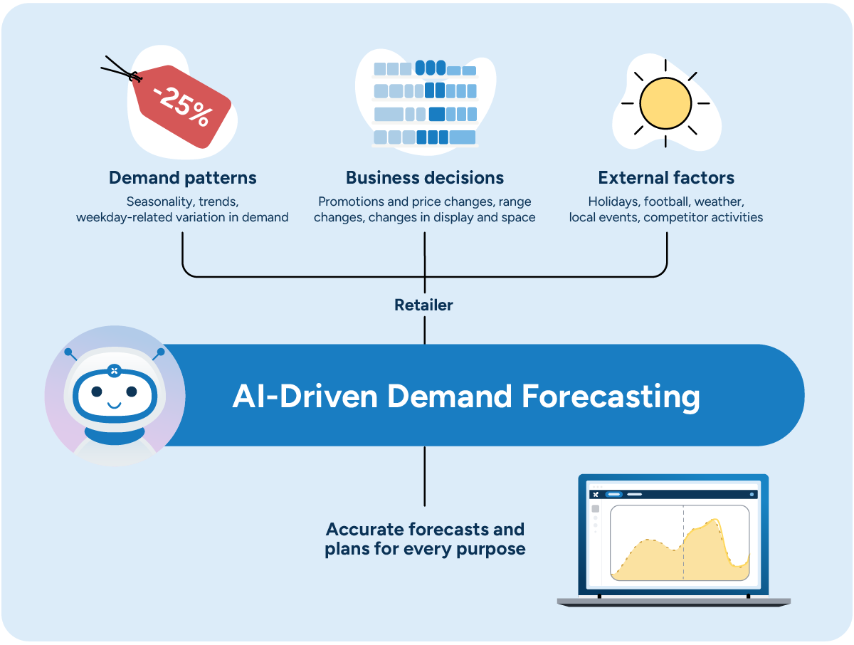
Traditional forecasting methods struggle to identify complex demand patterns when multiple factors influence sales simultaneously. Manual identification of these patterns is time-consuming and often incomplete.
RELEX’s machine learning engine automatically detects these systematic variations, such as seasonality, trends, and weekday patterns, enabling fast analysis and informed action. The system typically delivers 2-5 percentage point accuracy improvements over traditional time-series methods while ensuring consistency across thousands of products.
Incorporating business decisions
Internal business decisions, such as promotions, price changes, and assortment modifications, directly impact demand but are often poorly integrated with forecasting systems.
RELEX’s unified data model captures all demand drivers in a single system, automatically reflecting planned change into new forecasts. The system learns from historical data to understand how different promotion types, price discounts, and marketing activities affect demand. This creates transparent forecasts that separate the baseline demand, promotional impacts, and event-driven changes, allowing planners to evaluate the realism of promotional forecasts and identify when assumptions need adjustment.
Handling external factors
External factors, such as weather, holidays, and local events, significantly influence demand but are often overlooked or handled through crude manual adjustments.
RELEX ingests external data via API integrations, ERP connections, or CSV uploads to incorporate weather forecasts, holiday calendars, and event schedules. For recurring events with historical data, forecasting can be highly automated.
The system also identifies highly weather-sensitive products and enables automatic adjustments for near-term decisions. When unexpected events occur, such as products going viral on social media, planners can flag these and cleanse historical data to prevent anomalies from distorting future forecasts.
Scaling across portfolios
Traditional systems often require products to be segmented with different models applied to each segment, creating a maintenance burden and discontinuity when products move between segments.
RELEX’s machine learning engine handles all products without requiring segmentation. Because the system’s forecast error and bias in batch metrics are scale-agnostic, the same threshold values work whether a product sells 1 unit or 1,000 units per day. This delivers consistent accuracy improvements across entire portfolios while allowing planners to focus on exceptions rather than managing different forecasting approaches.
Enabling continuous improvement
Forecast models naturally become outdated as demand patterns evolve, new products are introduced, and market conditions change. Black-box systems make it difficult to identify why forecasts are failing, while overly complex systems require specialized expertise to modify and improve.
RELEX provides transparency into forecast components:
- Baseline forecasts
- Weekday patterns
- Weather impacts
- Promotional effects
- Special events
- Manual adjustments
This allows planners to quickly identify error sources. The RELEX Configuration Kit enables organizations to modify forecasting logic and test new approaches without vendor support. Combined with regular machine learning model updates that incorporate learnings from over 400 customer implementations, this ensures forecast accuracy improves continuously rather than degrading over time.
Turning demand forecasting insights into action
Measuring forecast accuracy only creates value when it drives better decisions. Here’s how to translate accuracy metrics into operational improvements.
When accuracy is poor but predictable
Sometimes low accuracy is simply the reality for certain products or situations. Knowing when to expect it allows planners to adapt accordingly.
When low accuracy is expected, planners can adapt in a few practical ways:
- Adjust safety stock and planning buffers rather than attempting to perfect inherently uncertain forecasts. Understanding where and when accuracy will be low enables strategic risk analysis of over- and under-forecasting consequences, allowing for better-informed business decisions. For instance, seasonal items that reliably achieve 60% accuracy but follow consistent patterns remain predictable, even if the precise volumes are uncertain.
- Position inventory centrally at distribution centers rather than committing stock to individual stores early. This allows allocation based on real-time demand signals as the season develops, maximizing sell-through at full price even with moderate forecast accuracy.
A real-world example of this is a fast-moving consumer goods (FMCG) manufacturer with a structured process for identifying “stars” in its portfolio of new products. “Star” products have the potential to break the bank, but they’re rare and seen only a couple of times each year. As the products have limited shelf life, the manufacturer does not want to risk potentially inflated forecasts driving up inventory “just in case.” Instead, they ensure they have production capacity, raw materials, and packaging supplies to deal with a scenario where the original forecast is too low.
When bias is detected
Systematic over- or under-forecasting requires immediate action at multiple levels. Small biases compound at aggregate levels. Even a 2% bias at the store level can create significant DC inventory imbalances.
Don’t wait to understand the root cause before taking action. If systematic bias is detected, adjust near-term orders proportionally while investigating the cause. For example, if forecasts have been consistently underestimating demand by 5%, temporarily increase order quantities to rebuild inventory positions before stockouts occur.
Once immediate actions are in place, conduct root cause analysis by investigating common sources of bias:
- Check if promotions were cancelled or modified. Was a large purchase order placed because the forecast contained a planned promotion that was later removed? If so, the root cause for poor forecast accuracy was not the forecasting itself but rather a lack of synchronization in planning.
- Review manual forecast adjustments. Manual adjustments often introduce systematic bias without planners realizing it. Monitor the added value of these changes on a continuous basis.
- Validate baseline demand assumptions. Has there been an ongoing trend that the forecasting models haven’t captured? Are seasonal patterns shifting? Has a competitor’s action permanently affected a company’s market share? Confirm that the fundamental demand patterns on which the models rely still accurately reflect current market conditions.
Once the source of bias is identified, retrain models or adjust parameters to fix it systematically. If promotional forecasts consistently overestimate lift, recalibrate those models. If manual adjustments consistently push forecasts in one direction, address why planners feel the need to override the system.
The need for predictable forecast behavior is also why extreme caution should be exercised when using machine learning algorithms. For example, when testing promotion data, an approach that is, on average, slightly more accurate than others might be discarded if it’s significantly less robust and more difficult for the average demand planner to understand.
Occasional extreme forecast errors can be detrimental to performance when the planning process has been set up to tolerate a certain level of uncertainty. These errors also reduce demand planners’ confidence in the forecast calculations, significantly hurting efficiency.
Forecast accuracy case studies and real-world examples
Ultimately, measuring forecast accuracy only matters if it leads to better decisions. These real-world examples show how retailers use forecast accuracy insights to adapt planning strategies, balance availability and inventory, and improve outcomes across different product segments.
Europris: Centralized forecasting drives segment-specific improvements
Norwegian discount variety retailer Europris demonstrates how centralized, automated forecasting can deliver different benefits across product segments. Before implementing RELEX, store managers spent three to four hours weekly on manual ordering without data analysis or forecasting support. The lack of visibility made it difficult to measure availability or understand why some stores carried significantly more inventory than others while still experiencing stockouts.
By centralizing replenishment with RELEX and applying sophisticated forecasting across their entire portfolio, Europris achieved 17%+ reduction in DC inventory within 18 weeks and improved store availability from 91% to 97%+. Store managers saw ordering time drop by 85%, freeing them to focus on customer care and merchandising. The automated system now handles the complexity of matching forecasts to individual store needs without manual categorization, allowing the supply chain team to focus their attention where human expertise adds the most value.
Ametller Origen: Tailoring strategies by product characteristics
Catalan grocery chain Ametller Origen Group illustrates how different product segments require different approaches based on their accuracy profiles and business impact. Facing rapid 19% year-over-year growth, the retailer needed greater inventory control as their supply chain complexity increased, particularly for fresh products where forecast errors quickly translate into waste or lost sales.
After implementing RELEX forecasting and replenishment, Ametller Origen achieved differentiated improvements across segments: 12 percentage point availability increase for non-perishables with 9 percentage point inventory reduction, compared to 4 percentage point availability increase for refrigerated goods with 24 percentage point inventory reduction. The retailer also drove a 14% increase in non-perishable sales and achieved significant reductions in fresh spoilage rates — a critical outcome for their commitment to sustainable business practices and CO2 neutrality by 2027.
Leverage forecast accuracy to deliver business results
Measuring forecast accuracy is essential, but results suffer when companies optimize the wrong things. Hitting accuracy targets does not guarantee success, while modest accuracy can deliver exceptional business results when measurement is focused where it matters most.
Success depends on three principles:
- Choose metrics that match the planning processes. Select the right aggregation level, weighting, and timing for each purpose, and use multiple metrics together. How metrics are calculated matters as much as which metrics are chosen.
- Use forecast accuracy to drive action, not reporting. Focus measurement where accuracy affects decisions, tolerate error where it does not, and address the real constraint, whether that is bias, limited flexibility, or another planning bottleneck.
- Rely on technology that improves continuously. Modern ML-based forecasting delivers measurable accuracy gains over traditional methods, while integrated planning turns those gains into better decisions, greater transparency, and ongoing improvement.
RELEX brings all three together. Our customers achieve industry-leading forecast accuracy while reducing waste, improving availability, and optimizing inventory because they measure the right things — and act on what they learn.
Measuring forecast accuracy FAQ
What is forecast accuracy, and why does it matter?
Forecast accuracy measures how closely demand predictions match actual sales, informing decisions from inventory ordering to staff scheduling. Poor accuracy creates cascading effects including stockouts, excess inventory, increased waste, and declining labor efficiency.
What is the difference between forecast accuracy and forecast bias?
Forecast accuracy measures the average size of errors regardless of direction, while forecast bias reveals whether forecasts are systematically too high or too low. Both must be tracked together to fully understand forecast performance and take appropriate action
What is a good level of forecast accuracy?
There is no universal benchmark because achievable accuracy depends on sales volume, demand variability, and forecast horizon. High-volume, stable products typically reach 75-85%, slow-moving items often fall between 50-70%, and fresh, weather-sensitive products generally land around 70-80%.
Why can aggregated forecast accuracy metrics be misleading?
Errors from individual products that are over- and under-forecasted can cancel each other out at the aggregate level, creating the illusion of high accuracy while hiding meaningful item-level bias. This is why accuracy should be measured at the same granularity as the planning decisions being made.
Should forecast accuracy improvements apply to all products equally?
No, efforts should focus on products where accuracy has the greatest business impact, such as fresh items, high-value goods, and volatile demand patterns. For low-value, low-frequency items, tolerating higher error thresholds is more efficient than investing resources in marginal accuracy gains.
Written by